Weights of Evidence Method
Weights of evidence is a quantitative method for combining evidence in support of a hypothesis. The method was originally developed for a nonspatial application in medical diagnosis, in which the evidence consisted of a set of symptoms and the hypothesis was of the type "this patient has disease x". For each symptom, a pair of weights was calculated, one for presence of the symptom, one for absence of the symptom. The magnitude of the weights depended on the measured association between the symptom and the pattern of disease in a large group of patients. The weights could then be used to estimate the probability that a new patient would get the disease, based on the presence or absence of symptoms. Weights of evidence was adapted in the late 1980s for mineral potential mapping with GIS. In this situation, the evidence consists of a set of exploration datasets (maps), and the hypothesis is "this location is favourable for occurrence of deposit type x". Weights are estimated from the measured association between known mineral occurrences and the values on the maps to be used as predictors. The hypothesis is then repeatedly evaluated for all possible locations on the map using the calculated weights, producing a mineral potential map in which the evidence from several map layers is combined. The method belongs to a group of methods suitable for multi-criteria decision making.
Similar to the methods of multiple regression in statistics, the weights of evidence model for combining evidence involves the estimation of response variable (favourability for mineral deposits) and a set of predictor variables (exploration datasets in map form). The terminology for weights of evidence has differed somewhat in the various publications written about it. In this document for the computer package Arc-WofE the following terms are used.
(1) Evidential theme. This is a map or area layer (in either vector or raster format -- shape or grid file) used for prediction of point objects (mineral occurrences). The polygons or grid cells of the evidential themes have two or more values (class values). For example, a geological map may have two or more values representing the classes (map units) present. Although weights of evidence was originally defined for binary evidential themes (also named binary patterns in several publications), it can also be applied to themes with more than two classes. Frequently, multi-class evidential themes will be generalized (simplified) by combining classes to a small number of values, facilitating interpretation.
(2) Training points. This is a point layer consisting of the locations at which the point objects are known to occur. Thus in mineral exploration, the points are the mineral deposits (showings, occurrences, etc.) previously discovered by prospectors, mappers, and exploration companies. But in other studies, the point objects may consist of locations of seismic events, intersections of faults, locations of springs, and others point types. The set of point locations is used to calculate the weights for each evidential theme, one weight per class, using the overlap relationships between the points and the various classes on the theme. The characteristics of the training points are held in an attribute table. Point subsets may be selected using the values of attributes, such as deposit size, or deposit type. However, points are treated as being either present or absent in the model, and are not weighted by characteristics such as deposit size.
(3) Unit cell. Each training point is assumed to occupy a small unit area, named the unit cell. In order to calculate the probability of a point occurrence, a unit of area must be selected. The output from weights of evidence is a map showing the probability that a unit area contains a point. Thus the values of probability will change with the choice of unit cell area. The unit cell is a constant set at the beginning of a particular computer run, and is the same for all training points and evidential themes. The area of the unit cell is unrelated to the physical size or influence of points, and is independent of the grid cell size used in raster datasets. The values of the weights are relatively independent of unit cell area, if the unit area is small.
(4) Response theme. This is an output map that expresses the probability that a unit area contains a point, estimated by combining the weights of the predictor variables (evidential themes). The response map is usually classified into a small number of values and depicted as relative favourability. If the training points are mineral deposits of a particular type, then the response map shows an estimate of mineral potential (also known as mineral prospectivity).
(5) Exploration dataset. Here we refer to digital datasets, such as digitized geological maps, geophysical images, geochemical survey data and remotely sensed images, frequently employed by exploration geologists in the mineral exploration process. There is always a process of extracting evidence from the raw dataset to be used in prediction. This process depends strongly in the exploration model being used.
(6) Exploration model. There are a large number of deposit models that have been defined for the various mineral deposit types, based on deposit characteristics. Deposit models help to classify and identify new occurrences, lead to an improved understanding of how the deposits formed, and act as an aid to exploration. However, they are usually based on characteristics of the deposit and its immediate surroundings, and many of the characteristic diagnostics of a mineral deposit type cannot be used with regional exploration datasets. The exploration model, on the other hand, refers to the characteristics of a deposit type identifiable in regional datasets, as used in the exploration process. It is important to note that the absence of evidence can be equally important as the presence of evidence and data on negative associations between deposits and particular types of data are often poorly documented.
(7) Study area theme (grid). In Arc-WofE the study area is a binary theme that defines the region of interest. It acts as a mask and areas of evidential themes and training points outside the study area are ignored in the calculations of weights and output maps.
Quantitative Mineral Potential Mapping in GIS
Although this computer package has been designed specifically for mineral potential mapping, it can also be used for other types of spatial prediction in which the goal is to predict the probability of occurrence of point objects. The remarks in this section are in the language of mineral exploration, but the same general principles guide other applications.
The GIS-based mineral potential mapping process can be broken down into four main steps: (1) building a spatial digital database, (2) extracting predictive evidence for a particular deposit type, based on an exploration model, (3) calculating weights for each predictive map (evidential theme), and (4) combining the evidential themes to predict mineral potential.
This computer package assumes that step 1 has already been completed. This may have been carried out in totally different GIS or image processing environments, not necessarily ARC/INFO or ArcView. Step 2 may have at least partially been done prior to using weights of evidence. However, parts of step 2 and all of step 3 are done within Arc-WofE, and comprise in many ways the most useful part of a mineral potential study. This is because the examination of the spatial relationships between the training points and evidential themes is exploratory, yielding measurements of spatial associations that are often unexpected. The process of generalization, grouping classes of evidential themes together, and identifying breaks in continuous variables that maximize spatial associations, often leads to a better understanding of the data. Finally, in step 4, a map showing combined evidence is valuable for identifying areas for exploration follow-up. In this step, maps showing a measure of confidence in the results, based on the uncertainty due the variances of weights, and uncertainty due to missing data (incomplete surveys), facilitate interpretation.
Weights of evidence is normally applied to exploration situations in which there is an adequate number of mineral deposits or occurrences already discovered that can be used as a set of training points for calculating weights. However, the package has also been designed to allow the user to calculate weights based on no "real" training point data set: the training set can be imaginary, and the overlap relationships between "points" and the selected evidential themes is decided arbitrarily by the user. This leads to weights governed by "expert" opinion. In all other respects the treatment of the problem is the same, so that if a user decides that the training points are not an adequate sample of the deposits actually present in the area, the weighting of the evidential themes can be based one expert judgment instead of statistical associations. This is advantageous for developing perhaps a variety of scenarios for different weights schemes, reflecting differences of opinion amongst experts, and allows the evaluation of sensitivity of the mineral potential maps to such differences. In fact there is a close mathematical similarity between weights of evidence and the 'likelihood ratios' (LS and LN) used to weights evidence in the original Prospector system, an expert system developed in the 1970s and 1980s for evaluating mineral prospects (McCammon, 1989).
In the following section, the basis of the weights of evidence model is outlined. However, readers should refer to other publications for a full explanation, e.g. Bonham-Carter et al. (1988), Agterberg et al. (1988), Agterberg and Bonham-Carter (1989), Wright (1996), Bonham-Carter et al. (1989), Bonham-Carter (1994), Wright and Bonham-Carter (1996).
| Next | Section Contents | Home |
Weights of evidence model
The WofE model can be applied to evidential themes with binary (presence/absence) classes, or to multi-class maps. Binary evidence is relatively straightforward to interpret, and the early publications on weights of evidence used mostly binary maps. Exploration geologists frequently deal with binary exploration datasets, as for example in separating anomaly from background in geochemistry. Interpreting weights and combining evidential themes is easier with binary data than with multi-class data. Also, weights calculated for a small number of classes are more robust than ones calculated using a large number of classes, and this is particularly critical when a relatively small number of points are in the training data. Binary themes produce weights with smaller variances, and are therefore more stable.
Binary Evidential Themes
Figure 1 shows a rectangular view with an evidential theme with two classes (value 2 for presence, value 1 for absence), and a set of training points. In Figure 1A, the boundary of a base map theme is shown, and in Figure 1B the base map is shown to have acted as a "cookie-cutter", masking out some of the evidential theme, and some of the training points.
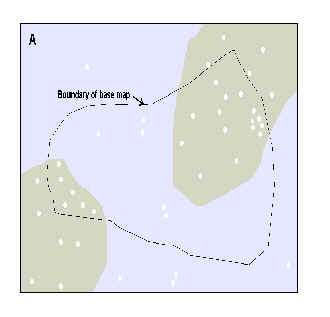
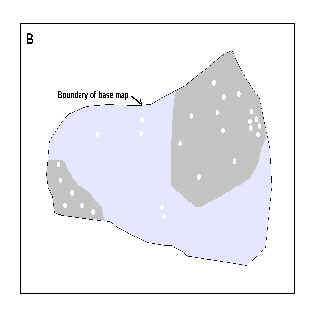
Figure 1. A. Rectangular area showing binary evidential theme and training points. B. Same area trimmed back to study area base map, excluding both points and areas outside study area.
Given the area of the unit cell is
u km2, the area of the base map in unit cells is A(T)/u=N(T), where T is the
base map, A() denotes area,
and N() denotes a count of the number of unit cells -- not
restricted to integer numbers. Then within the base map, the
number of training points is denoted as N(D).
In this instance, N(D) is
always an integer number, and independent of u. Suppose the
evidential theme is denoted by B, A(B)/u
= N(B) is the area in
unit cells of the region (either vector polygons or grid cells)
where B is present (class value=2, for example). Similarly, ![]() is the area in
unit cells where B is absent (class value = 1, for example). If
there is no missing data,
is the area in
unit cells where B is absent (class value = 1, for example). If
there is no missing data, ![]() . However, if there are regions within T
where B is unknown (e.g. incomplete survey), another class (often
value=0) is employed and
. However, if there are regions within T
where B is unknown (e.g. incomplete survey), another class (often
value=0) is employed and ![]() . We will assume that N(missing)
= 0 for the time being.
. We will assume that N(missing)
= 0 for the time being.
Using the GIS, we can readily
measure N(T), N(B) and ![]() . We can also count the number of training points of B and on
. We can also count the number of training points of B and on![]() , denoted as
, denoted as ![]() and
and ![]() , respectively.
, respectively.
The weights provide a measure of spatial association between the points and the evidential theme. A weight is calculated for each class of the evidential theme. A positive value of the weight indicates that there are more points on that class than would occur due to chance; conversely a negative value indicates that fewer points occur than expected. A value of zero, or very close to zero, indicates that the training points are distributed randomly with respect to that class. For binary maps with only two classes (the labeling of class by a value is arbitrary), W+ is used for the weights where the evidential theme is present (value=2 in this instance), W- is used for the weights sign, except if they both equal zero. The difference between the weights is know as the contrast, C. Thus C=W+ - W-. The contrast is an overall measure of spatial association between the training points and the evidential theme, combining the effects of the two weights. Sometimes, W+ can be close to zero, yet W- is strongly negative. This situation arises if the presence of the theme is not particularly predictive of training points, but the absence of the theme provides strong evidence that points are unlikely to occur. Conversely there can be an imbalance between the absolute values of W+ and W- in the other direction; or the two weights can have absolute values in about the same range.
In general, absolute weights values between 0 and 0.5 are mildly predictive; values between 0.5 and 1 are moderately predictive; values between 1 and 2 are strongly predictive, and greater than 2 are extremely predictive.
For the derivation of weights, see
Bonham-Carter (1994, ch. 9). In general, the weights for binary
themes are given by the ratio of the following conditional
probabilities:
![]() and
and
![]()
where P() denotes probability and ln denotes natural logarithms. It is assumed that probabilities are estimated as simple area proportions, so that
![]() ,
,
![]() ,
,
![]() and
and
![]() .
.
where ![]() is the number of training points on theme
B, etc.
is the number of training points on theme
B, etc.
The following working formula for W+ is
![]()
and similar expression for W-. It is interesting to note that if the area of the unit cell becomes very small, this expression approximately satisfies
![]()
where W+* denotes W+ for a small unit cell, because N(B) and N(T) become very large and the number of training points are negligible in comparison. Thus the W+* value is the natural logarithm of what has been termed the 'normalized density' of points (Elliot et al., 1992), where the normalized density (ND) is the ratio
![]()
The values of normalized density (percent points/ percent area) and W+* are shown in Table 1.
Table 1. Relationship between normalized density and weight when unit cell is very small.
Points - Theme Association |
W+* | ND |
positive |
>0 |
>1 |
none |
0 |
1 |
negative |
<0 |
0-1 |
Note that the normalized density is Equal to exp(W+*), and is therefore similar to the sufficiency ratio(LS) as used in the original Prospector expert system. It should also be noted that the weights are not very sensitive to units cell area, and as the unit cell becomes small, W+ approaches the value of W+*.
| Next | Section Contents | Home |
Probability Considerations
If the prior probability per unit area that the region occupied by the study area contains a deposit is assumed to be constant equal to the training points density, N(D)/ N(T), then the posterior probability of a deposit given one or more evidential themes will either increase or decrease (as compared to the prior probability). Given one evidential theme, the posterior probability, P(D|B), can be calculated from the prior probability, P(D) by
![]()
This is Bayes' rule. It is convenient to transform the expression from probability units to logits, where logits are the natural logarithms or odds, and odds are related to probability by O = P/(1/P). If we write L() for logits, then the posterior logit of deposit per unit area given a single evidential theme is:
![]()
if the binary theme is present or
![]()
if the theme is absent. We speak of the prior logit being "updated" by the evidence to yield the posterior logit. This is the loglinear form of Bayes' rule. By making an assumption of conditional independence (to be discussed later, and see Bonham-Carter, 1994, ch. 9) two evidential themes (B1 and B2) can be used to update the prior logit to the posterior logit. If the evidential themes are binary, this leads to four possible situations, depending on the possible combinations of the themes:
![]() ,
,
![]() ,
,
![]() and
and
![]() .
.
Similarly, 3 or more binary evidential themes may be combined by adding the appropriate weights according to the presence or absence of the themes at each location, and assuming conditional independence.
The advantage of using the loglinear model over the ordinary probability expression is that the weights are easier to interpret than probability factors. Because a positive weight implies that the (evidential theme-training points) association is greater than would be expected due to chance, it is relatively easy to understand the results. The calculation of the posterior logit is easy to follow (and program) because adding weights together is similar to the intuitive approach for combining evidence based on common sense. The fact that using the loglinear scale allows one to add weights is convenient. Usually, one converts the mapped logit values back to probability for map display, although this is often unnecessary because the rank ordering of posterior probabilities is the same as the ordering of posterior logits. Thus if a quantile classification is applied to the mapped output values, and the same colour scheme used, probability and logit maps will be the same. Posterior logits, (e.g. L(D|B) are converted to probabilities by the expression
![]()
| Next | Section Contents | Home |
Multi-class Evidential Themes
Most exploration datasets result at least initially in thematic maps that consist of more than 2 map units. Geological maps, even after they have been simplified, usually comprise several units. Geophysical and geochemical maps are classified into multiple classes, corresponding either to colours or contour levels on an intensity scale. It is often possible to groups map units (or class values) together in a reclassification or generalization step, but sometimes it is better to retain at least a modest number of classes as a multi-class evidential theme rather than using a binary one. As mentioned previously, having too many classes results in less robust estimates of the weights. One the other hand, new multi-class themes may reflect the real picture of favourable or unfavourable evidence with more precision.
Table 2. Variation of weights of evidence with cumulative distance from anticline axes. The contrast, C, reaches a maximum value at class 5 (1.25 km). The area of the unit cell is 1 km2, and the area units are in terms of unit cells. The point column is the number of cells containing a point. s(W+) is the standard deviation of W+, and s(W-) is the standard deviation of W-. Addition of an extra column (not shown here) containing the Studentized contrast (C/s(C)) is also helpful for choosing the cutoff distance, because it shows the contrast relative to the uncertainty due to the weights. (From Bonham-Carter, 1994, ch. 9)
| Class | Distance | Area | Points | W+ | s(W+) | W- | s(W-) | C |
| 1 | <0.25 | 260 | 15 | .949 | .266 | -.160 | .139 | 1.109 |
| 2 | 0.50 | 617 | 30 | .770 | .187 | -.353 | .164 | 1.123 |
| 3 | 0.75 | 813 | 37 | .700 | .168 | -.471 | .181 | 1.171 |
| 4 | 1.00 | 998 | 43 | .643 | .156 | -.596 | .201 |
1.237 |
| 5 | 1.25 | 1280 | 51 | .561 | .143 | -.820 | .244 | 1.381 |
| 6 | 1.50 | 1497 | 54 | .458 | .139 | -.883 | .269 | 1.341 |
| 7 | 1.75 | 1643 | 55 | .381 | .137 | -.850 | .279 | 1.231 |
| 8 | 2.00 | 1848 | 57 | .296 | .135 | -.845 | .303 | 1.142 |
| 9 | 2.25 | 2009 | 59 | .246 | .132 | -.887 | .335 | 1.133 |
| 10 | 2.50 | 2133 | 60 | .202 | .131 | -.862 | .355 | 1.064 |
| 11 | 2.75 | 2229 | 61 | .173 | .130 | -.869 | .380 | 1.042 |
| 12 | 3.00 | 2343 | 61 | .122 | .130 | -.693 | .380 | 0.815 |
| 13 | 3.25 | 2403 | 61 | .096 | .130 | -.586 | .380 | 0.682 |
| 14 | 3.50 | 2444 | 61 | .079 | .130 | -.505 | .381 | 0.584 |
| 15 | 3.75 | 2495 | 61 | .057 | .130 | -.396 | .381 | 0.453 |
| 16 | 4.00 | 2531 | 61 | .043 | .130 | -.310 | .381 | 0.352 |
| 17 | 4.25 | 2560 | 61 | .031 | .130 | -.235 | .382 | 0.265 |
| 18 | 4.50 | 2607 | 61 | .013 | .130 | -.103 | .382 | 0.116 |
| 19 | 4.75 | 2633 | 62 | .019 | .129 | -.176 | .412 | 0.194 |
| 20 | 5.00 | 2654 | 62 | .011 | .129 | -.103 | .413 | 0.114 |
| 21 | 5.25 | 2695 | 62 | -.005 | .129 | .054 | .413 | -0.060 |
| 22 | 5.50 | 2715 | 62 | -.013 | .129 | .140 | .414 | -0.153 |
| 23 | 5.75 | 2728 | 62 | -.017 | .129 | .202 | .414 | -0.219 |
| 24 | 6.00 | 2757 | 63 | -.012 | .127 | .166 | .453 | -0.178 |
| 25 | >6.00 | 2942 | 68 |
| Next | Section Contents | Home |
Map Combination
An important concept used in WofE is the idea of a "unique conditions" table and associated "unique conditions" map. This step is carried out in grid format in WofE, regardless whether the evidential themes were input as shape or grid files, but the concept applies equally in vector mode. The unique conditions table and map are produced by an overlay of the evidential themes selected for prediction.
A unique condition is the collection of polygons or grid cells at which the same combination of the evidential themes occurs on the overlay map. Each row of the unique conditions table corresponds to a unique set of class values, with the same characteristics as indicated by the row vector of class values, one column for each evidential theme. If the evidential themes are all binary, then the maximum number of unique conditions equals 2n, where n is the number of themes. However, the number of unique conditions rises sharply if some of the evidential themes are multi-class. The following table illustrates the concept for a combination of 3 binary these, producing a map with 8 unique conditions.
Table 3. Unique condition table for three binary themes, in which class values are 2=present, 1=absent.
| UC Number | Area, km2 | Theme 1 | Theme 2 | Theme 3 |
| 1 | 101.7 | 2 | 2 | 2 |
| 2 | 56.2 | 2 | 2 | 1 |
| 3 | 142.1 | 2 | 1 | 1 |
| 4 | 17.0 | 1 | 2 | 2 |
| 5 | 29.8 | 1 | 1 | 2 |
| 6 | 229.3 | 1 | 2 | 1 |
| 7 | 171.2 | 2 | 1 | 2 |
| 8 | 3.8 | 1 | 1 | 1 |
In the corresponding unique conditions map, the values are the unique conditions number.
The weights of evidence calculations are carried out on the unique conditions table within WofE, and posterior probability and other values are added as new fields. The unique conditions map can then be classified and displayed using one of the new calculated fields. The code also is designed so that unique conditions table can be exported for analysis in other software packages, if the need arises. The table with new fields of calculated values may then be reimported for display and analysis.
| Next | Section Contents | Home |
Conditional Independence Test
WofE allows the user to carry out a pair-wise conditional independence test, and an "omnibus" test as described in Bonham-Carter (1994, ch. 9).
Confidence Maps
One of the standard outputs from WofE is a map of confidence in the posterior probability. This is the ratio of the posterior probability to its standard deviation. High values of this ratio indicate that the uncertainty is relatively small compared to the probability value itself, whereas low values (that may be in areas of low or high probability) indicate relative large uncertainty.
The uncertainty always includes the uncertainty of the weights. If some evidential themes contain areas with missing information (incomplete surveys), the variances due to missing information is included. Calculation of these values is described in Agterberg et al. (1988).
Agterberg, F.P. and Bonham-Carter, G.F., 1990, Deriving weights of evidence from geoscience contour maps for the prediction of discrete events: Proceedings 22nd APCOM Symposium, Berlin, Germany, v.2, p. 381-395.
Agterberg, F.P., Bonham-Carter, G.F, and Wright, D.F., 1990, Statistical pattern integration for mineral exploration: In Computer applications in Resource Estimation: Predictions and Assessment for Metals and Petroleum, Eds. G. Gaal and D.F. Merriam, Pergamon, Oxford, p. 1-21.
Bonham-Carter, G.F., 1994, Geographic Information Systems for Geoscientists: Modeling with GIS: Pergamon, Oxford, 398 p.
Bonham-Carter, G.F., Agterberg, F.P. and Wright, D.F., 1988, Integration of geological datasets for gold exploration in Nova Scotia: Photogrammetric Engineering and Remote Sensing, v. 54(11), p. 1585-1592.
Bonham-Carter, G.F., Agterberg, F.P. and Wright, D.F., 1989, Weights of evidence modeling: a new approach to mapping mineral potential: In Statistical Applications in the Earth Sciences, Eds. F.P. Agterberg and G.F. Bonham-Carter, Geological Survey of Canada, Paper 89-9, p. 171-183.
Elliot, J.E., Wallace, C.A., Lee, G.K., Antweiler, J.C., Lidke, D.J., Rowan, L.C., Hanna, W.F., Trautwein, C.M., Dwyer, J.L. and Moll, S.H., 1992, Mineral resource assessment map for vein and replacement deposits of gold, silver, copper, lead, zinc, manganese and tungsten in the Butte 1 degree x 2 degree quadrangle, Montana: U.S.Geological Survey, Miscellaneous Investigations Series, Map I-2050-D, 31p.
McCammon, R.B., 1989, Prospector II - the redesign of Prospector: AI Systems in Government, March 27-31, 1989, Washington, D.C., p. 88-92.
Wright, D.F., 1996, Evaluating volcanic hosted massive sulphide favourability using GIS-based integration models, Snow Lake area, Manitoba: Ph.D. Dissertation, University of Ottawa, 344 p.
Wright, D.F. and Bonham-Carter, G.F., 1996, VHMS favourability mapping with GIS-based integration models, Chisel Lake-Anderson Lake area: In EXTECH I: A Multidisciplinary Approach to Massive Sulphide Research in the Rusty Lake-Snow Lake Greenstone Belts, Manitoba, Eds. G.F. Bonham-Carter, A.G. Galley and G.E.M. Hall, Geological Survey of Canada, Bulletin 426, p. 339-376, 387-401.
| Next | Top of Section | Home |