Define Fuzzy Membership
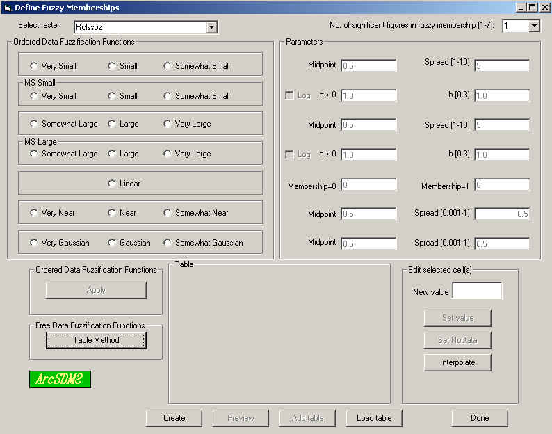
This tool has been completely redesigned to use functions to define the fuzzy membership for ordered and a table for free data. The Ordered Data Fuzzification Functions and their associated parameters use mathematical functions to transform the input data to the desired fuzzy membership in the interval [0,1]. Some of these functions do not work with negative values or values of zero; so it is required to transform or reclassify your data to positive values before fuzzification. A linear transform made with the Map Calculator is often the easiest way to do this transform to positive numbers. Fuzzification can be thought of as the process of assigning fuzzy membership values to crisp values. The Free Data Fuzzification Functions are used with free or categorical data and essentially involve editing a table. It is necessary to define the number of significant figures that will be used for the fuzzy membership function. Once the fuzzy membership function is defined it can be previewed in a graph and stored in a table, which can be reloaded for use again. This table is often a useful way to further edit the fuzzy membership for free data where the user may be interested in considering other data while defining the fuzzy membership. The Define Fuzzy Membership window is shown below. Following the window is an outline of the steps to define a fuzzy membership function and definitions of all the functions.
Fuzzification of Ordered and Categorical Data
Ordered data indicates a raster for which the value attribute is some sort of measurement. The value attribute has a meaning and can be used for meaningful computations. Some of these functions do not work with negative values or values of zero; so it is often useful to transform your data to a positive values before fuzzification. To create a fuzzy membership raster follow the following steps:
1. Select the raster in the "Select raster" scrolling window at the top left of the window.
2. Define how many significant figures are desired. If number of significant figures is 1, then the input values will be integers between [0,10]. If the number of significant figures is 2, then the input values will be integers between [0,100]. The inputs are always integers with appropriate of number of figures. The output, when the fuzzy membership raster is created, will always be a floating point number between [0,1] with the number of significant figures selected by the user. The default number of significant figures is 1, which will create a fuzzy membership raster with values such as 0.3 by entering 3.
3. For Ordered data click the radio button for the desired fuzzification function and type in the desired parameters for that functions. This will activate the Apply button in the Ordered Data Fuzzification Functions. The method of Categorical data is discussed below.
4. Click the Apply button in the Ordered Data Fuzzification Functions. The mapping of the input values from the selected raster to the fuzzy membership values will appear in the Table subwindow as shown below. In this case, two significant figures for a large function was selected with the midpoint at 9 and a spread of 5. The fuzzy membership value (FMemShp) for an input of 5 and 9 will be 0.05 and 0.90, respectively. The Preview button will be activated, as shown below.
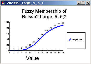
5. If the Preview button is clicked, a graph of the mapping of inputs to fuzzy membership will be displayed as shown below. This graph is first saved as a table with a default name that records the fuzzification function and the parameters. The table is required by ArcMap in order to create a graph. The table can also be reloaded later using the Load table button. In this case the input raster was Rclssb2, the large fuzzification function was selected, the midpoint was 9, the spread was 5, and the number of significant figures was 2. The graph can be closed by clicking the x in the upper right corner. The graphs can be reopened by clicking the ArcMap Tool menu and selecting Graphs. A list of all the graphs made will appear for selection.
6. As stated above a table created by the Preview button, can be reloaded later using the Load Table button.
7. The tabled fuzzy membership values can be edited using the Edit Selected Cells subwindow. Single or multiple rows in the data can be edited simultaneously. Also, interpolation between start and stopping values can be done. To edit the fuzzy membership for value 6, which is 11.64 in the last view of this window above, click on the row with the desired value. The selected row will be highlighted in blue. Enter the new value in the New Value window, such as 13. Then click Set Value. The new value will appear in the fuzzy membership column for the selected row.
To interpolate between two value, for example between the value 1 fuzzy membership of 0.00 and the new value 6 fuzzy membership of 13 as shown in the above window, do the following: Click on the first row, the starting the the interpolation interval. Holding down the left button click on the last row of the interpolation interval. In the example below the first and sixth rows were selected. Then click the Interpolate button, which will linearly interpolate between the beginning and ending fuzzy membership values. In this case between 0 and 13 over values 1 to 6.
After editing a function, it is wise to save the values in a table. This is done by clicking Preview to create a table and graph.
8. For Categorical Data, the Table method is used to assign fuzzy memberships. The method of entering data is the same as editing data discussed in item 7 above. The descriptor attribute for the Categorical will be displayed on the right side of the Table window as guidance. For categorical data is is useful to replace the Count column with the names of each row. This attribute can be selected in the drop-down window with the word Count in the above picture. For example is a categorical shape file with a categorical attribute "Code" were used to create a raster, the resulting raster would have a "Code" attribute containing the names. This attribute can be displayed in place of the Count attribute to guide the selection of fuzzy memberships.
9. After getting the desired fuzzy membership function, the new fuzzy membership raster can be calculated by clicking the Create button. This will first open the Fuzzy Logic Model Tables window shown below. If the user has multiple fuzzy logic models, select the desired model, such as Flmdl1 in the window below. If a new model is being created, click the "Make and add a new table row" and the creation of a new raster with a default name will be completed. The new fuzzy membership raster will be added to the table of contents with the name starting with FM. After FM will be the name of the input raster. For example, in this example the input raster was rclssb2; so the fuzzy membership raster will be FMrclssb2. Note this is a temporary raster. The user can delete it or make it permanent by right clicking on the raster name in the table of contents and selecting the Make Permanent option.
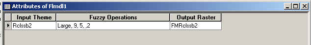
The Fuzzy Logic Model Tables window below is part of a mechanism to record the fuzzy logic processing steps to ease documentation. This window creates a table in which all processing for a model is stored. The default name of the table is Flmdl# for fuzzy logic model with a sequential number. This fuzzy model table is added to the table of contents and can be opened to see a record of the model, as shown in the Attribute table below. With a fuzzy model with many processing steps will get quite long. This Fuzzy Logic Model Table can have additional steps appended to it as the modeling proceeds or multiple Fuzzy Logic Model Tables can be used to develop multiple models in parallel. This same table will also store the Fuzzy Logic calculations.
10. When the fuzzification is completed click the Done button to close the Window. Note: The results of this fuzzification process is stored as a temporary file in the ~sdmtemp folder with the actual name raster#. It is a good practice to make these temporary files into a permenant file, give them a useful name, and store them in your working folder. This will facilitate recovery of your work, if you should loose the MXD document.
Definition of Fuzzification Functions
Fuzzication functions include the small, large, near, gaussian, mean-standard deviation large (MS large), and mean-standard deviation small (MS small) functions. In addition two hedges, very and somewhat are used to modify these function. These functions are discussed in Tsoukalas nd Uhrigh (1997) and Lou and Dimitrakopoulos (2003).
The two hedges implemented are very and somewhat (Tsoukalas and Uhrig,1997). Very is also known as concentration. The hedge functions are the fuzzy membership squared, a decreasive function, or the square root of the fuzzy membership, an increasive function. The hedges are normally called Very and Somewhat. Thus Very Small, which implies smaller than small, is Small squared; where as Very Large, which is larger than Large, is the square root of Large. So the function applied to the hedge depends on the semantic implication. The appropriate function for the semantic meaning of the hedge is applied automatically. The user can always verify that the appropriate selection has been made by Previewing the results.
The fuzzification algorithms small and large are used to indicate that small or large values of the crisp set aree larger members of the fuzzy set (Tsoukalas and Uhrig,1997). The spread and mid parameters are subjectively defined to reflect the expert opinion. Examples of the small and large functions and hedges are shown in Figure 2. Small and Large do not work with negative values or values of zero; so the user must transform the data to a positive values before fuzzification. The small fuzzification algorithm is defined as
Where f1 is the spread of the transition from a membership value of 1 to 0 and f2 is the mid point where the membership value is 0.5 (Tsoukalas and Uhrig, 1997).
The large fuzzification algorithm is defined as
Where f1 is the spread of the transition from a membership value of 1 to 0 and f2 is the mid point where the membership value is 0.5 (Tsoukalas and Uhrig, 1997).
Note this function works improperly for negative crisp values. To apply these functions to negative numbers, the crisp values need to be transformed or reclassified to positive numbers before fuzzification.
Figure 2: Examples of small and large fuzzification using a mid value of 5 and a spread of 3.
Mean-Standard-Deviation Small (MS Small) and Mean-Standard-Deviation Large (MS Large) are from Lou and Dimitrakopoulos (2003). These functions are similar to the Small and Large function with the mid-point and spread controlled by the mean and standard deviation of the data. By clicking a radio button, the Log to the base 10 can be taken before the mean and standard deviation are calculated. The Log cannot, of course, be used if the values are zero or negative. This is often useful for very skewed data, which is normalized by taking the log. The MS Small function is
The MS Large function is
Where m = the mean, s = the standard deviation, a = a multiplier of the mean, and b = a multiplier of the standard deviation.
Examples of MS Small and MS Large and hedges are shown below in Figure 3. In this example for MS Small the mean is 30, the standard deviation is 20, and both a and b are 1. For MS Large, the mean is 20, the standard deviation is 20, and both a and b are 1. The user can change the a and b values to scale the effect of the mean and standard deviation.
Figure 3: Examples of small and large fuzzification using a mid value of 5 and a spread of 3.
The fuzzification function near is used when some intermediate crisp value is
the larger member of the fuzzy set (Tsoukalas
and Uhrig,1997). The spread and mid parameters are subjectively
defined to reflect the expert opinion. Near does
not work with negative values or values of zero; so the user must transform the
data to a positive values before fuzzification. An example of the near algorithm is given
in Figure 4
. The near function is also known as a sinusoidal membership function (Burrough
and McDonnell, 1998). The near fuzzification algorithm is defined as
![]()
Where f1 is the spread of the transition from a membership value of 1 to 0 and f2 is the mid point where the membership value is 0.5 (Tsoukalas and Uhrig, 1997).
Figure 4: Example of near fuzzification using a mid value of 10 and a spread of 0.3.
The fuzzification function Gaussian is similar to the near function but has a more narrow spread (Tsoukalas and Uhrig,1997). Gaussian does not work with negative values or values of zero; so the user must transform the data to a positive values before fuzzification. The Gaussian fuzzification algorithm is defined as
![]()
Where f1 is the spread of the transition from a membership value of 1 to 0 and f2 is the mid point where the membership value is 0.5 (Tsoukalas and Uhrig, 1997).
![]()
Combination fuzzification functions can be made by applying multiple fuzzification functions to a integer-grid table and then editing the table to piecewise combine the different functions. An example of just a process using the two near functions is shown in Figure 5
Figure 5: Example of a combination of two near functions with spread of 0.9, a mid value of 5 for less than 5, a mid value of 15 for greater than 15, and a membership value of 1 between 5 and 15.
The selection of the appropriate spread value is a subjective process that is dependent on the range of the crisp values. A useful way to experiment with different spread values is to use a spreadsheet program with graphs. These graphs can be quickly made using the DBF tables created by the Preview button. Then a picture of the effects of different spread functions can be quickly developed. Note as shown in Figure 6 and Figure 7 as the spread gets smaller the fuzzy memberships approach zero more slowly.
Figure 6: Examples of a range of spreads for a small function with a constant mid value of 5.
Figure 7: Examples of a range of spreads for a near function with a constant mid value of 50.
Lou, X., and Dimitrakopoulos, R., 2003, Data-driven fuzzy analysis in quantitative mineral assessment: Computers and Geosciences, v. 29, p. 3-13.
Tsoukalas, L.H., and Uhrig, R.E., 1997, Fuzzy and neural approaches in engineering: New York, John Wiley and Sons, Inc., 587p.
| Next | Section Contents | Home |
![]()